Small-plot analysis

library(CBADASReml)
#> Loading required package: asremlPlus
#> ASReml-R needs to be loaded if the mixed-model functions are to be used.
#> 
#> ASReml-R is available from VSNi. Please visit http://www.vsni.co.uk/ for more information.
#> Loading required package: ggplot2
#> Loading required package: gstat
#> Loading required package: sf
#> Linking to GEOS 3.13.0, GDAL 3.8.5, PROJ 9.5.1; sf_use_s2() is TRUE
library(asreml)
#> Loading required package: Matrix
#> Online License checked out Fri Aug 22 12:51:01 2025
#> Loading ASReml-R version 4.2

CBADASReml

Introduction

A typical type of experimental analysis that this package will assist with is the small plot trial. Here we will show the general workflow for performing a small-plot analysis and how each function from the package can be used. Analysis of small plot trials is done using linear mixed-effects models (LMMs), using {ASReml} or {glmmTMB}, and this package contains helper functions for this type of modelling.

Note that the trial design is not handled at all by this package, and we recommend the use of {speed} or {FielDHub} for creating small plot trial designs.

Mathematical Background

Let:

$$\begin{equation*} y = X b + Z u + e \end{equation*}$$

Where

• $y \in \mathbb{R}^{n}$ is the vector of observations.
• $b \in \mathbb{R}^{p}$ is the vector of fixed effects.
• $X \in \mathbb{R}^{n \times p}$ is the design matrix for the fixed effects.
• $u \in \mathbb{R}^{q}$ is the vector of random effects.
• $Z \in \mathbb{R}^{n \times q}$ is the design matrix for the random effects.
• $e \in \mathbb{R}^{n}$ is the vector of residuals.

It is assumed that the vectors $u$ and $e$ are independent, and their joint distribution is a multivariate Gaussian described by:

$$\begin{equation*} \begin{bmatrix} u \\ e \end{bmatrix} \sim N \bigg( \begin{bmatrix} 0 \\ 0 \end{bmatrix} , \begin{bmatrix} G & 0 \\ 0 & R \end{bmatrix} \bigg) \end{equation*}$$

Where $G$ and $R$ are covariance matrices for $u$ and $e$ and are functions of the variance parameters $\sigma_g$ and $\sigma_r$, and finally the dependent variable $y$ is described by:

$$\begin{equation*} y \sim N \big( X b , Z G Z^\intercal + R \big) \end{equation*}$$

These $G$ and $R$ covariance matrices, or covariance structures, are very important. These represent the way the random effects and the residuals behave, and $\sigma_g$ and $\sigma_r$, the covariance structure parameters are the things we try and estimate when we use ASReml.

In the case of independent and identically distributed (IID) residual structures, the residual covariance parameter $\sigma_r$ will be some variance component $\sigma_e^2$.

Exploratory Data Analysis

After gathering data from an experiment, it is useful to perform an exploratory data analysis on the raw data, and for this you will likely use a combination of tidyverse and gplot2 for this, to visualise outliers, the data distribution, etc. in order to get a preliminary grasp of what you are working with, and to observe the data for any issues that will hinder the actual analysis. As an assistance with this process, the function exploratory_table is provided.

CBADASReml::exploratory_table(
    data = oats,
    response = "yield",
    groupby = c("Variety", "Nitrogen")
)
#>        Variety Nitrogen             mean median               sd
#> 1  Golden_rain    0_cwt               80     75 21.0047613649858
#> 2  Golden_rain  0.2_cwt             98.5  102.5 13.4721935853075
#> 3  Golden_rain  0.4_cwt 114.666666666667    110 29.9443929086343
#> 4  Golden_rain  0.6_cwt 124.833333333333  129.5 20.8750249500849
#> 5   Marvellous    0_cwt 86.6666666666667   92.5 16.5730705262081
#> 6   Marvellous  0.2_cwt            108.5  111.5 26.8533051969399
#> 7   Marvellous  0.4_cwt 117.166666666667  118.5 9.78604448521805
#> 8   Marvellous  0.6_cwt 126.833333333333  122.5 20.2920345620311
#> 9      Victory    0_cwt             71.5     65   20.59854363784
#> 10     Victory  0.2_cwt 89.6666666666667   89.5 22.5092573548455
#> 11     Victory  0.4_cwt 110.833333333333    106 26.0108951531213
#> 12     Victory  0.6_cwt            118.5  114.5 30.0915270466622
#>                  cv reps min max     range
#> 1  26.2559517062322    6  60 117  60 - 117
#> 2  13.6773538937132    6  82 114  82 - 114
#> 3  26.1142961412508    6  86 161  86 - 161
#> 4  16.7223163819105    6  96 149  96 - 149
#> 5  19.1227736840862    6  63 105  63 - 105
#> 6  24.7495900432626    6  70 140  70 - 140
#> 7  8.35224280388454    6 104 132 104 - 132
#> 8  15.9989760016014    6  99 156  99 - 156
#> 9   28.809151941035    6  53 111  53 - 111
#> 10  25.103260990534    6  64 130  64 - 130
#> 11 23.4684768298838    6  81 157  81 - 157
#> 12 25.3936937102634    6  86 174  86 - 174

Model Fitting and Validation

We may use the R package asreml as follows to implement an LMM. For the purpose of this vignette we will fit a few different models, so we can demonstrate different techniques from the package.

# The needs to be ordered so that the model can run
oats <- oats[order(oats$Column), ]

mod_oats <- asreml(
    fixed = yield ~ Variety + Nitrogen + Variety:Nitrogen,
    random = ~ idv(Blocks) + idv(Blocks):id(Wplots),
    residual = ~ ar1(Column):ar1(Row),
    data = oats,
    trace = FALSE
)
#> Warning in asreml(fixed = yield ~ Variety + Nitrogen + Variety:Nitrogen, : Some
#> components changed by more than 1% on the last iteration

mod_oats <- update(mod_oats, aom = TRUE)

mod_rats <- asreml(
    fixed = weight ~ littersize + Sex + Dose,
    random = ~idv(Dam),
    residual = ~units,
    data = rats,
    trace = FALSE
)

mod_rats <- update(mod_rats, aom = TRUE)

In the first model, mod_oats, we are using the oats data:

Data

• The oats data has 72 rows, 2 treatments (Nitrogen and Variety), and plots (3 levels) within blocks (6 levels). Therefore:
  • $n = 72$ (number of observations)
  • $p = 3$ (number of fixed effects, including an interaction effect)
  • $q = 2$ (number of random effects, blocks, and plots within blocks)

$y$

• yield is our $y \in \mathbb{R}^{72}$ ($72 \times 1$) vector.

$X$

• Variety, Nitrogen and their interaction Variety:Nitrogen are in the $X \in \mathbb{R}^{72 \times 3}$ ($72 \times 3$) matrix.

$b$

• There are 3 fixed effects which are continuous, therefore our fixed effects vector is given by $b \in \mathbb{R}^{3 \times 1}$

$Z$

• Blocks and Blocks:Wplots make up our $Z \in \mathbb{R}^{n \times q}$ matrix. Since these are factors, each level is treated as it’s own dummy variable. We end up with two $Z_i$ matrices which make up $Z = [ \; Z_1 \; Z_2 \; ]$ which are given as follows (if ordered by their respective variables):

$$\begin{equation*} Z_{1} = \begin{bmatrix} 1 & 0 & 0 & 0 & 0 & 0 \\ \vdots \times \text{10} & 0 & 0 & 0 & 0 & 0 \\ 1 & 0 & 0 & 0 & 0 & 0 \\ 0 & 1 & 0 & 0 & 0 & 0 \\ 0 & \vdots \times \text{11} & 0 & 0 & 0 & 0 \\ & & \vdots & & & \end{bmatrix} \in \mathbb{R}^{72 \times 6} \end{equation*}$$

$$\begin{equation*} Z_{2} = \begin{bmatrix} 1 & 0 & 0 & 0 & 0 & 0 & 0 & 0 & 0 & 0 & 0 & 0 & 0 & 0 & 0 & 0 & 0 & 0 \\ \vdots \times \text{2} & 0 & 0 & 0 & 0 & 0 & 0 & 0 & 0 & 0 & 0 & 0 & 0 & 0 & 0 & 0 & 0 & 0 \\ 1 & 0 & 0 & 0 & 0 & 0 & 0 & 0 & 0 & 0 & 0 & 0 & 0 & 0 & 0 & 0 & 0 & 0 \\ 0 & 1 & 0 & 0 & 0 & 0 & 0 & 0 & 0 & 0 & 0 & 0 & 0 & 0 & 0 & 0 & 0 & 0 \\ 0 & \vdots \times \text{2} & 0 & 0 & 0 & 0 & 0 & 0 & 0 & 0 & 0 & 0 & 0 & 0 & 0 & 0 & 0 & 0 \\ & & & & & & & & \vdots & & & & & & & & & \end{bmatrix} \in \mathbb{R}^{72 \times 18} \end{equation*}$$

Where each column in $Z_1$ represents the $6$Blocks, and the columns in $Z_2$ represent the $6 \times 3 = 18$Blocks $\times$Wplots.

$u$

• Since we have $2$ model terms (idv(Blocks) and idv(Blocks):id(Wplots)), we have two $Z_i$ matrices, and also two $u_i$ vectors. Our random effects vector is given by:
  • $u = \begin{bmatrix} u_1 \\ u_2 \end{bmatrix}$
  • $u_1 \sim N(0, G_1) \in \mathbb{R}^{6}$
  • $u_2 \sim N(0, G_2) \in \mathbb{R}^{18}$.

$G$

• idv(Blocks) + idv(Blocks):id(Wplots) is the random effects variance structure. Since we have two terms, we again have two $G_i$’s. We specify the idv variance model function, which is the homogeneous scaled identity variance structure, i.e. $\sigma^2 I$. The second term has a /direct product/ implied by the : operator, which in the case of matrices is a /Kronecker product/, of idv(Blocks) and id(Wplots). id variance model means it is simply a correlation structure, i.e. $I$, and there is no estimation of a variance parameter. Noting we have 2 random effects terms:
  • $G_1 = \sigma_1^2 I_6$ ($I_6$ is the $6 \times 6$ identity matrix)
  • $G_2 = (\sigma_2^2 I_6) \otimes I_3$
  • $G = \bigoplus_{i = 1}^2 G_i = \begin{bmatrix} \sigma_1^2 I_6 & 0 \\ 0 & (\sigma_2^2 I_6 \otimes I_3) \end{bmatrix}$

$e$

• The error vector is specified by the single model term ar1(Column):ar1(Row), therefore the error is given by:
  • $e \sim N(0, R)$ where $R$ is the $R$ structure

$R$

• ar1(Column):ar1(Row) specifies the residual variance structure. In this case we refer to an autoregressive model of order 1 (AR(1)) on both Row and Column, where the : operator implies a separable Kronecker product structure. The variance model ar1 is of the form: $\Sigma_{ii} = 1, \Sigma_{ij} = \phi \Sigma_{i-1, j}, i > j+1, \lvert \phi \rvert < 1$.
  • $R = \Sigma_c(\phi_c) \otimes \Sigma_r(\phi_r)$
  • Where $\phi$ refers to the correlation within the columns ($\phi_c$) or the rows ($\phi_r$).

In the second model, mod_rats, we are using the rats data:

• weight is our $y$ vector.
• littersize, Sex and Dose are in the $X$ matrix.
• Dam is in the $Z$ matrix. We specify the idv variance model function, which is the homogeneous scaled identity variance structure, i.e. $\sigma^2 I$. In other words, the term is IID:
  • $u \in \mathbb{R}^d \sim N(0, G)$
  • $Z$ is the design matrix for Dam.
  • $G = \sigma_d^2 I_d$.
• idv(units) is the residual variance structure, in this case the residual term has the homogeneous covariance matrix: $\sigma^2 I$. This is basically saying all observations have the same error distribution (IID):
  • $e \in \mathbb{R}^n \sim N(0, R)$
  • $R = \sigma_e^2 I_n$

Upon executing the above in R, the ASReml-R code will attempt to estimate the variance components $\sigma_d^2$ and $\sigma_e^2$, using the REML algorithm.

Function examples

Traditional Diagnostics (ASReml-R)

plot.asreml

plot(mod_oats)

plot of chunk plot_mod_oats

plot(varioGram(mod))

plot(varioGram(mod_oats))

plot of chunk variogram_mod_oats

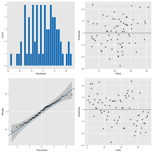
CBADASReml Diagnostics

outlier_summary

The purpose of the outlier_summary function is to observe potential outliers that can then be discussed with the data provider. Below is an example for the rats dataset that is included within ASReml-R.

outlier_summary(mod_rats)
#> 
#> ── Outliers detected: 2 ────────────────────────────────────────────────────────
#>    Dose Sex littersize Dam weight units combined_trt residuals
#> 56    C   F         13   5   5.02    56       13_F_C -4.090506
#> 66    C   F          9   6   3.68    66        9_F_C -7.941340
#> 
#> ── Data table ──
#> 
#>     Dose Sex littersize Dam weight units combined_trt  residuals
#> 56     C   F         13   5   5.02    56       13_F_C -4.0905065
#> 57     C   F         13   5   6.04    57       13_F_C -1.4769901
#> 53     C   F         13   5   7.16    53       13_F_C  1.3927533
#> 55     C   F         13   5   7.14    55       13_F_C  1.3415079
#> 54     C   F         13   5   7.09    54       13_F_C  1.2133944
#> 129    C   F         13  10   5.92   129       13_F_C -1.1145276
#> 126    C   F         13  10   6.67   126       13_F_C  0.8050510
#> 128    C   F         13  10   6.53   128       13_F_C  0.4467297
#> 130    C   F         13  10   6.52   130       13_F_C  0.4211353
#> 125    C   F         13  10   6.44   125       13_F_C  0.2163802
#> 131    C   F         13  10   6.44   131       13_F_C  0.2163802
#> 127    C   F         13  10   6.43   127       13_F_C  0.1907859
#> 66     C   F          9   6   3.68    66        9_F_C -7.9413397
#> 64     C   F          9   6   7.26    64        9_F_C  1.3727706
#> 65     C   F          9   6   6.58    65        9_F_C -0.3963900

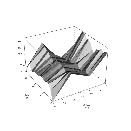
directional_variograms

The purpose of this function is to view the autocorrelation structure in both directions, rather than the traditional approach with ASReml-R.

plot(directional_variograms(mod_oats))

plot of chunk directional_variograms_mod_oats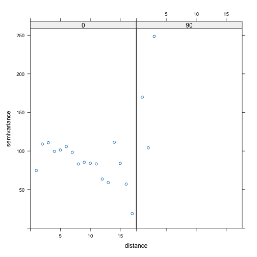

Model Outputs

Traditional Outputs (ASReml-R)

wald

For getting the significance of each variable in the model

wald(mod_rats)
#> Wald tests for fixed effects.
#> Response: weight
#> Terms added sequentially; adjusted for those above.
#> 
#>               Df Sum of Sq Wald statistic Pr(Chisq)    
#> (Intercept)    1   1477.67         8981.5 < 2.2e-16 ***
#> littersize     1      4.58           27.8 1.312e-07 ***
#> Sex            1      9.80           59.5 1.199e-14 ***
#> Dose           2      3.76           22.8 1.100e-05 ***
#> residual (MS)         0.16                             
#> ---
#> Signif. codes:  0 '***' 0.001 '**' 0.01 '*' 0.05 '.' 0.1 ' ' 1

predict

predict.asreml(mod_oats, classify = "Nitrogen")
#> $pvals
#> 
#> Notes:
#> - The predictions are obtained by averaging across the hypertable
#>   calculated from model terms constructed solely from factors in
#>   the averaging and classify sets.
#> - Use 'average' to move ignored factors into the averaging set.
#> - The simple averaging set: Variety
#> - The ignored set: Blocks,Wplots
#> 
#>   Nitrogen predicted.value std.error    status
#> 1    0_cwt        77.76388  6.929776 Estimable
#> 2  0.2_cwt       100.15097  6.896569 Estimable
#> 3  0.4_cwt       114.41044  6.887489 Estimable
#> 4  0.6_cwt       123.22901  6.912904 Estimable
#> 
#> $avsed
#>  overall 
#> 3.748427

CBADASReml Outputs

anova_table

Show an ANOVA table for multiple models, with p-values for each effect against each response.

rats[["newresp"]] <- rats[["weight"]] * runif(nrow(rats))

mod_rats2 <- asreml(
    fixed = newresp ~ littersize + Sex + Dose,
    random = ~idv(Dam),
    residual = ~units,
    data = rats,
    trace = FALSE
)

mod_rats2 <- update(mod_rats2, aom = TRUE)

anova_table(mod_rats, mod_rats2)
#>       Effect weight newresp
#> 1 littersize      0   0.804
#> 2        Sex      0   0.208
#> 3       Dose      0   0.008

pred_table

Get the mean for each level of a fixed effect, as well as standard error, and confidence intervals.

pred_table(mod_rats, classify = "Dose")
#> Error:
#> ! Classify must be type character

Least significant difference

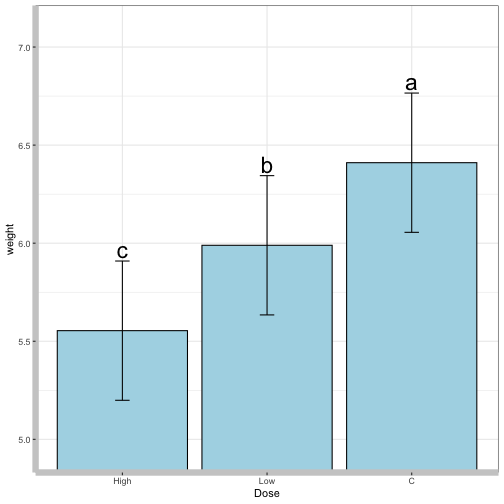
lsd_table

Show a least significant difference table:

lsd_table(mod_rats, classify = "Dose")
#>   treatment group      lsd    means
#> 1         C     a 0.354997 6.410370
#> 2       Low     b 0.354997 5.989315
#> 3      High     c 0.354997 5.554064

lsd_graph

Show an LSD graph of the same data:

lsd_graph(mod_rats, classify = "Dose")

plot of chunk lsd_graph_mod_rats