Using nert to augment agricultural analytics with SMIPS data
Russell Edson and Max Moldovan
Source:vignettes/nert_for_agricultural_analytics.Rmd
nert_for_agricultural_analytics.RmdThe nert package provides straightforward and seamless access to the TERN Soil Moisture Integration and Prediction System (SMIPS) datasets, which include soil moisture estimates that can be used in your data analytics pipelines. This document showcases this process with the example of a synthesised multi-site grain production experiment. The nert package is loaded and used to download soil moisture time series data at various locations across South Australia. Recognising soil moisture as a classical confounder—affecting crop yield (via root-zone water availability) and nitrogen treatment (via increased volatilisation in moist soils)—we will augment our modelling of the grain production to use soil moisture estimates over the treatment period for estimating the nitrogen treatment effect.
A synthetic dataset for a grain production experiment
A simulated dataset containing yield data for a fictitious grain
production experiment has been included with the nert
package. The dataset is called grain, and you can load the
package and this dataset with:
library(nert)
data(grain)
str(grain)
#> 'data.frame':    2880 obs. of  10 variables:
#>  $ Site             : Factor w/ 10 levels "Adelaide","Barossa Valley",..: 1 1 1 1 1 1 1 1 1 1 ...
#>  $ Latitude         : num  -34.9 -34.9 -34.9 -34.9 -34.9 ...
#>  $ Longitude        : num  139 139 139 139 139 ...
#>  $ SowDate          : Date, format: "2022-05-20" "2022-05-20" ...
#>  $ NitrogenDate     : Date, format: "2022-06-04" "2022-06-04" ...
#>  $ Rep              : Factor w/ 3 levels "1","2","3": 1 1 1 1 1 1 1 1 1 1 ...
#>  $ Variety          : Factor w/ 8 levels "Variety_A","Variety_B",..: 1 1 1 1 1 1 1 1 1 1 ...
#>  $ Nitrogen_kgNha   : Factor w/ 4 levels "0","30","60",..: 1 1 1 2 2 2 3 3 3 4 ...
#>  $ SeedRate_plantsm2: Factor w/ 3 levels "75","150","300": 1 2 3 1 2 3 1 2 3 1 ...
#>  $ Yield_Tha        : num  3 3.69 3.89 2.76 3.27 ...
The grain dataset supposes that a hypothetical grain
production experiment has been run at a selection of ten sites across
South Australia, investigating the effects of four different treatment
levels of nitrogen application and three different seeding rates on the
grain yield for some crop with eight varieties.
Note that we have locational coordinates (in Latitude
and Longitude) for each of the sites, as well as dates for
the crop sowing and nitrogen applications (in SowDate and
NitrogenDate respectively.) This spatio-temporal
information is useful, as it allows us to match up the experimental
sites with the data points that we need to download from SMIPS.
Download SMIPS data for the sites across times
Here we use the nert package to download SMIPS soil
moisture datasets from the TERN Data Portal, which we can use to augment
our analysis of the grain experiment data. The two key
SMIPS datasets of interest are:
totalbucket: an estimate of the volumetric soil moisture (in units of mm) from the SMIPS bucket moisture store,SMindex: the SMIPS soil moisture index (i.e., a percentage between 0 and 100 that indicates how full the SMIPS bucket moisture store is relative to its 90cm capacity).
For simplicity, suppose we are interested in the SMIPS soil moisture
index (SMindex) data, for all days falling between the
earliest nitrogen application date up to 30 days after the last
application date, and we want the soil moisture index at each site (by
latitude/longitude coordinates). We can generate this date range in a
straightforward way using the NitrogenDate column of the
grain dataset as follows:
start_date <- min(grain$NitrogenDate)
end_date <- max(grain$NitrogenDate) + 30
date_range <- seq(start_date, end_date, by = "1 day")

c(date_range[1], date_range[length(date_range)])
#> [1] "2022-05-07" "2022-07-15"
We also need the latitude and longitude for the sites, which we can
readily retrieve from the grain dataset columns
Latitude and Longitude:
sites <- unique(grain[, c("Site", "Latitude", "Longitude")])
sites
#>                    Site  Latitude Longitude
#> 1              Adelaide -34.94773  138.6244
#> 289      Barossa Valley -34.54843  138.9580
#> 577        Clare Valley -33.83754  138.6012
#> 865      Eyre Peninsula -34.37378  135.7967
#> 1153 Fleurieu Peninsula -35.52307  138.4608
#> 1441    Kangaroo Island -35.71041  137.0736
#> 1729    Limestone Coast -37.88957  140.6388
#> 2017         Sturt Vale -33.34666  140.0723
#> 2305        Murraylands -35.12425  139.3014
#> 2593    Yorke Peninsula -35.05124  137.2090
Now TERN supplies the SMIPS daily data rasters as cloud-optimised GeoTIFFs (or COGs), which contain the soil moisture point predictions across the entirety of Australia. However, because they are cloud-optimised, we can be clever in our downloading to make sure that we only download data for the locations of interest, rather than the entire raster. The nert package works in tandem with the terra package to achieve this efficiency:
- First, we download the information for a daily SMIPS raster
using
nert::read_smips, - Then we extract only the point values we need, using
terra::extract.
This leads to a quicker and tighter data download. The below code
shows this process. (Note that terra::extract is particular
about the order of the latitude/longitude coordinates: longitude should
be specified first, followed by latitude.)
smips_data <- data.frame()
for (i in seq_along(date_range)) {
  r <- read_smips(date = date_range[i], collection = "SMindex")
  smips_points <- terra::extract(
    x = r,
    y = data.frame(lon = sites$Longitude, lat = sites$Latitude),
    xy = TRUE
  )
  names(smips_points)[2] <- "smips_smi_perc"

  smips_data <- rbind(
    smips_data,
    data.frame(
      Date = date_range[i],
      Latitude = smips_points$y,
      Longitude = smips_points$x,
      smips_smi_perc = smips_points$smips_smi_perc
    )
  )
}
head(smips_data)
#>         Date  Latitude Longitude smips_smi_perc
#> 1 2022-05-07 -34.95253  138.6237     0.25906488
#> 2 2022-05-07 -34.55264  138.9537     0.17677850
#> 3 2022-05-07 -33.83285  138.6037     0.07674548
#> 4 2022-05-07 -34.37270  135.7944     0.53408158
#> 5 2022-05-07 -35.52237  138.4638     0.37496096
#> 6 2022-05-07 -35.71231  137.0741     0.30223876
We can add the Site column to the
smips_data to make it easier to use it in conjunction with
the grain dataset during the analysis:
smips_data$Site <- sites$Site
head(smips_data)
#>         Date  Latitude Longitude smips_smi_perc               Site
#> 1 2022-05-07 -34.95253  138.6237     0.25906488           Adelaide
#> 2 2022-05-07 -34.55264  138.9537     0.17677850     Barossa Valley
#> 3 2022-05-07 -33.83285  138.6037     0.07674548       Clare Valley
#> 4 2022-05-07 -34.37270  135.7944     0.53408158     Eyre Peninsula
#> 5 2022-05-07 -35.52237  138.4638     0.37496096 Fleurieu Peninsula
#> 6 2022-05-07 -35.71231  137.0741     0.30223876    Kangaroo Island
We are now ready to proceed with the analytics.
A simple model for grain yield
First, we model the grain yield with a simple model without taking into account any soil moisture confounding—that is, without reference to the SMIPS data that we have just downloaded. We will later incorporate the SMIPS data to see how including the soil moisture as a covariate improves the nitrogen treatment effect size estimates.
Here we will use the nlme package to fit a linear
mixed-effect model. The grain yield Yield_Tha will be
modelled taking the Variety, nitrogen application rate
Nitrogen_kgNha and seeding rate
SeedRate_plantsm2 as fixed terms, and incorporating the
Site and replicate (Rep) structure of the
experiment in a random effect term.
library(nlme)
simple_model <- lme(
  fixed = Yield_Tha ~ Variety * Nitrogen_kgNha * SeedRate_plantsm2,
  random = ~ 1 | Site / Rep,
  data = grain
)
We can check the confidence intervals for the effect sizes of the nitrogen treatments for this simple model:
simple_model.ints <- intervals(simple_model, which = "fixed")$fixed
simple_model.Neffects <- simple_model.ints[paste0("Nitrogen_kgNha", c(30, 60, 90)), ]
simple_model.Neffects
#>                        lower      est.     upper
#> Nitrogen_kgNha30 -0.17355028 0.0392950 0.2521403
#> Nitrogen_kgNha60  0.08045472 0.2933000 0.5061453
#> Nitrogen_kgNha90  0.09779306 0.3106383 0.5234836
Augmenting the yield model with soil moisture data
Next, we augment our modelling by including the SMIPS soil moisture
data as a covariate (perhaps anticipating that the soil moisture
improves the yield, but might reduce the effect of nitrogen applied to
the soil due to volatilisation). To keep things simple, for each site
(and its associated nitrogen application date) we take an average of the
SMIPS-reported soil moisture index from the date of the nitrogen
application until 30 days after the application, which we will store in
a new column called SoilMoisture_avg.
for (site in sites$Site) {
  start_date <- unique(grain[which(grain$Site == site), "NitrogenDate"])[1]
  dates <- seq(start_date, start_date + 30, by = "1 day")
  smips <- smips_data[which(smips_data$Site == site & smips_data$Date %in% dates), ]
  smips_avg <- mean(smips[["smips_smi_perc"]])
  grain[which(grain$Site == site), "SoilMoisture_avg"] <- smips_avg
}
We can then add this average soil moisture as a fixed effect to the linear mixed-effect model:
augmented_model <- lme(
  fixed = Yield_Tha ~ Variety * Nitrogen_kgNha * SeedRate_plantsm2
    + SoilMoisture_avg + SoilMoisture_avg:Nitrogen_kgNha,
  random = ~ 1 | Site / Rep,
  data = grain
)
The confidence intervals for the effect sizes of the nitrogen application treatments for this augmented model are then as follows:
augmented_model.ints <- intervals(augmented_model, which = "fixed")$fixed
augmented_model.Neffects <- augmented_model.ints[paste0("Nitrogen_kgNha", c(30, 60, 90)), ]
augmented_model.Neffects
#>                        lower      est.     upper
#> Nitrogen_kgNha30 -0.03984861 0.2000454 0.4399395
#> Nitrogen_kgNha60  0.31409573 0.5539898 0.7938838
#> Nitrogen_kgNha90  0.33961765 0.5795117 0.8194058
We can use ggplot2 plotting to graph the confidence intervals for the simple model versus the augmented model, and illuminate the difference attained when we include the soil moisture as a confounding term in our modelling:
library(ggplot2)

ci <- rbind(
  data.frame(simple_model.Neffects, model = "Simple Model"),
  data.frame(augmented_model.Neffects, model = "SMIPS-Augmented Model")
)
ci$term <- paste0("Nitrogen_kgNha", c(30, 60, 90))

pd <- position_dodge(-0.4)
ggplot(ci, aes(x = est., y = term, colour = model)) +
  scale_y_discrete(limits = rev) +
  geom_point(position = pd) +
  geom_errorbarh(aes(xmin = lower, xmax = upper), position = pd, height = 0.2) +
  labs(y = "predictor", x = "estimate")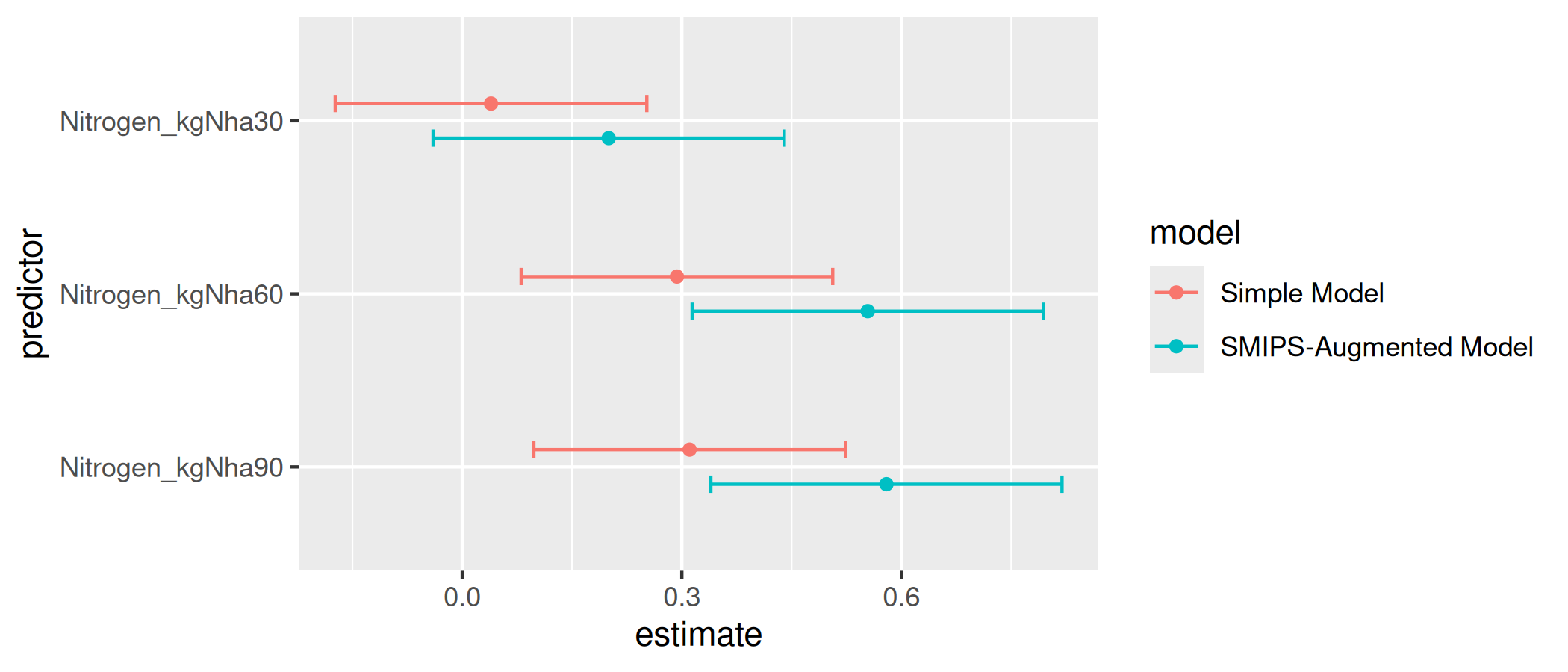
Nitrogen effect estimates compared between the simple model and the SMIPS-augmented model.
From the comparison of the effect sizes for the nitrogen treatment, we can see that ignoring the effect of soil moisture in the simple model underestimates the direct nitrogen treatment effect. The augmented model, in contrast, accounts for the soil moisture and the potential nitrogen volatilisation that may occur in higher soil moisture conditions.
Simplified collection with collect_tern_data()
The hand-written for loop above is shown for didactic
purposes — it makes the per-date COG read and per-site point extraction
explicit. For routine use, collect_tern_data() performs the
same operation vectorised across locations, with one COG open per
(dataset, date, variant) regardless of the number of points. The same
SMindex time series can be produced with a single call:
smips_dt <- collect_tern_data(
  xy = data.frame(lon = sites$Longitude, lat = sites$Latitude),
  date_range = c(start_date, end_date),
  datasets = "SMIPS",
  smips_collection = "SMindex",
  verbose = FALSE
)
head(smips_dt)
smips_dt is a data.table with one row per
(date, location); a single extraction call replaces the inner
terra::extract() of the loop. The example above is shown
with eval=FALSE to avoid duplicating the network traffic
already performed by the loop; the output schema is identical to
smips_data apart from the column name
(SMIPS_SMindex rather than
smips_smi_perc).